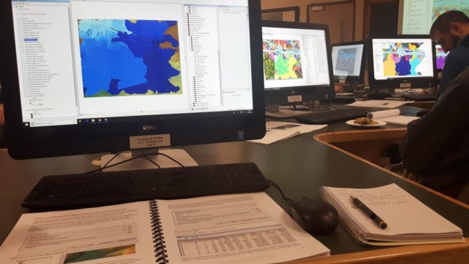
On the morning of the 25th of January, I headed down to the Forestry complex at the University of New Brunswick(UNB) to attend a LiDAR workshop that I had been looking forward to all week. For those that might not know, LiDAR stands for Light Detection and Ranging and refers to light reflection measurements that can be mapped to model the elevations in the landscape. LiDAR data can also be manipulated to create other analytics. On this particular day, we were going to be using the data to graph watershed delineations and overland flow modelling. Van Lantz, who is the Dean of Forestry and Environmental Management at UNB said the following:
We are very excited to be offering this professional training course this year. This is one of the first in a series of training oppurtunities the Faculty has planned in the areas of GIS, LiDAR, remote sensing and other related fields that can help natural resource professionals upgrade their knowledge and skills.
As I sat down in the laboratory in the IUC Forestry building, I was met with nostalgia from my time as a student at the University of Toronto, when I would spend hours in the GIS lab in the university basement. UNB provided students with a monitor workstation each. Our instructor was Jae Ogilvie who presented us with our name badges and a centimeter thick workbook from which we were to follow instructions. Whilst, Jae would be leading the class, we were given permission to work independently from the workbooks if we were so inclined. As I looked around, I met with people who were familiar and unfamiliar as well as younger and older than I. It was very refreshing to be in a classroom environment where people of all skill levels were here to learn.
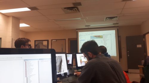
The first steps towards creating cool LiDAR maps was downloading the data set from the website. We then turned ‘Spatial Analyst’ in the ArcMap extensions on, so that the tools associated with it in the ArcMap toolbox could be used. We were provided with an overview model of what the process would look like. We first learned how to symbolize the data so that we could utilize it visually in the most efficient way. When visualizing LiDAR data, it is advisable to use color scales because it is a raster and the entire shapefile will look blank. As soon as the colors are changed, it is a beautiful image of landscapes emerging from a three dimentional image. Furthermore, the first data set used is called a DEM which stands for Digital Elevation Model which is where the data is showing the landscape in topographical way so that when elevations change drastically, the slope is visible as an indentation around the sloped area.
Jae Ogilvie, RPF, GISP who taught the course had the following to say:
The Faculty of Forestry & Environmental Management at UNB has recently endeavored into a series of 1 and 2-day workshops intended to empower land managers, decision makers and generally interested parties, using state-of-the-art technologies. Leveraging publicly available high resolution Light Detection and Ranging (LiDAR) and industry-standard Geographic Information Systems (GIS) software, workshops have been designed with different knowledge entry-points in mind. Focusing on hands-on exercises and practical tips & tricks, it is our hope that participants will come away with a better understanding of LiDAR as a technology, but more importantly the ability to work with these rich datasets to assist with their best management practices and land stewardship goals.
The course started out with inputting the provided DEM into a series of tools from the Spatial Analyst toolbox. First, we used the Fill tool in the hydrology toolset which created a filled DEM which exposes the intersurface, and floods the DEM so that bridges and culverts can be distinguished from DAMS. After this, we calculated the flow direction raster. To determine watershed delineation, the D8 algorithm was used which assigns one of eight directions to each raster cell. This tool can also be found in the hydrology toolset. Flow calculation was calculated by figuring out the upstream cell count, also from the hydrology toolset, as well as the next tool, flow accumulation. The DEM for flow accumulation appears when it is first calculated so it is smart to go into symbology and equalize the histogram.
We used the con tool from the conditional toolset to create a potential channel network raster. This means that the flow accumulation raster will be used to create streams or channels based on where the data suggests the flow is coming from. Going back to the hydrology toolset, we used stream link to improve the segmentation of channel reaches. After this, we vectorized potential channel network lines so that we could see them in an isolated environment. Then, we created ‘notches’ which are where water bodies connect to eachother and put it into a line shapefile by digitizing the lines. We redo all the previous steps but we use the notch lines to determine notched elevations.
Adam Taylor who is a GIS Analyst for Service New Brunswick, had the following to say about the event:
Mr. Jae Ogilvie gave superb instruction and demonstrated a lot of flexibility related to the procedures he showed the class. His documentation was very detailed and yet easy to follow, as well as being adaptable to many possible workflows. He was eager to help guide students with advice related to their specific data concerns. I would recommend the course to anyone interested in learning more about the subject.



Be the first to comment